Snakes and Ladders (Part 3 of 3): Analysing the classic children’s game

To recap the analysis from our previous article, we have now shown that the advantage to Player 1 in snakes and ladders is minimal (amounting to less than 6 extra wins out of every 1,000 games). In this post we look at visualising some results, focusing in particular on the distribution of game lengths and the frequency with which the 100 squares are landed on. Note that for simplicity we count any score above 100 as landing on square number 100.

We make a couple of alterations from our existing code in order to achieve this. First we need a variable to act as a counter of “ply” (a term borrowed from chess and other games, meaning the number of individual player moves, or half-turns), and then another variable to keep track of the frequency of visits to each square.

We also import Python’s default plotting package Matplotlib in order to generate the distributions of these variables later on.

import numpy as np
from collections import Counter
import matplotlib.pyplot as plt


def snakes_and_ladders(x):
    dict_sal = {21:3, 24:7, 35:9, 50:11, 53:15, 60:23,
                75:44, 89:48, 93:25, 97:65, 99:58,
                4:16, 12:33, 18:22, 26:37, 42:61,
                49:51, 55:74, 82:98, 85:95, 88:92}
    return dict_sal.get(x, x)

def roll_die(x):
    x += np.random.randint(1, 7)
    x = snakes_and_ladders(x)
    return x

p1_wins = p2_wins = 0
ply_count = Counter()
squares_count = Counter()

np.random.seed(42)

NUM_GAMES = 1000000

for games in range(NUM_GAMES):
    p1 = p2 = 0
    ply = 0
    while True:
        p1 = roll_die(p1)
        ply += 1
        if p1 > 100:
            squares_count[100] += 1
            p1_wins += 1
            ply_count[ply] += 1
            break
        else:
           squares_count[p1] += 1
        p2 = roll_die(p2)
        ply += 1
        if p2 >= 100:
            squares_count[100] += 1
            p2_wins += 1
            ply_count[ply] += 1
            break
        else:
            squares_count[p2] += 1

top_of_ladder = [16, 22, 33, 37, 51, 61, 74, 92, 95, 98]
tail_of_snake = [3, 7, 9, 11, 15, 23, 25, 44, 48, 58, 65]

ladder_tops = {k: squares_count[k] for k in top_of_ladder}
snake_tails = {k: squares_count[k] for k in tail_of_snake}
unmarked = {k: squares_count[k] for k in range(1, 101) if k not in top_of_ladder + tail_of_snake}

plt.bar(ladder_tops.keys(), ladder_tops.values(), 0.8, color="green", label="ladder top")
plt.bar(snake_tails.keys(), snake_tails.values(), 0.8, color="red", label="snake tail")
plt.bar(unmarked.keys(), unmarked.values(), 0.8, color="blue", label="unmarked")
plt.xlim([0, 101])
plt.ylim([0, 2500000])
plt.xlabel("Square")
plt.ylabel("Frequency")
plt.title("Distribution of Squares Landed On")
plt.legend(loc="upper right")
plt.draw()

plt.figure()
plt.bar(ply_count.keys(), ply_count.values(), 0.5, color="blue")
plt.xlim([0, 601])
plt.ylim([0, 18000])
plt.xlabel("Total Ply")
plt.ylabel("Frequency")
plt.title("Distribution of Half-Turns")
plt.draw()

plt.show()

The above code is available here.

The one piece of code that perhaps needs some explanation is the Counter container from Python’s collection module, which we use to track the squares landed on and the total number of half-turns. This is a subclass of a dict object but has the benefit of being able to use the increment operator even if the element is not already present.

We have also separated the squares into “ladder_tops”, “snake_tails”, and “unmarked” to allow us to plot the frequency of these different classes with different colours. We can see the effect of this here:

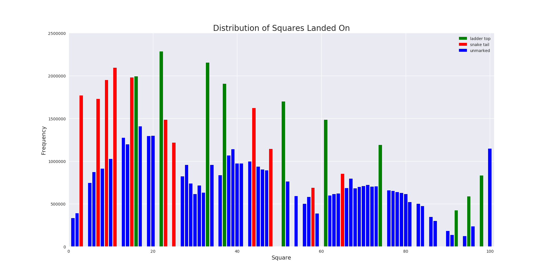
It is unsurprisingly clear to see that the snake and ladder squares are hit more frequently than their local unmarked squares. Note too that some squares are never “visited”. These correspond to ladder bases and snake heads, since the counters will always move away from these squares.

With some analysis offline we can discern that the most frequently visited square on this particular board is 22, whilst the least visited is 94.

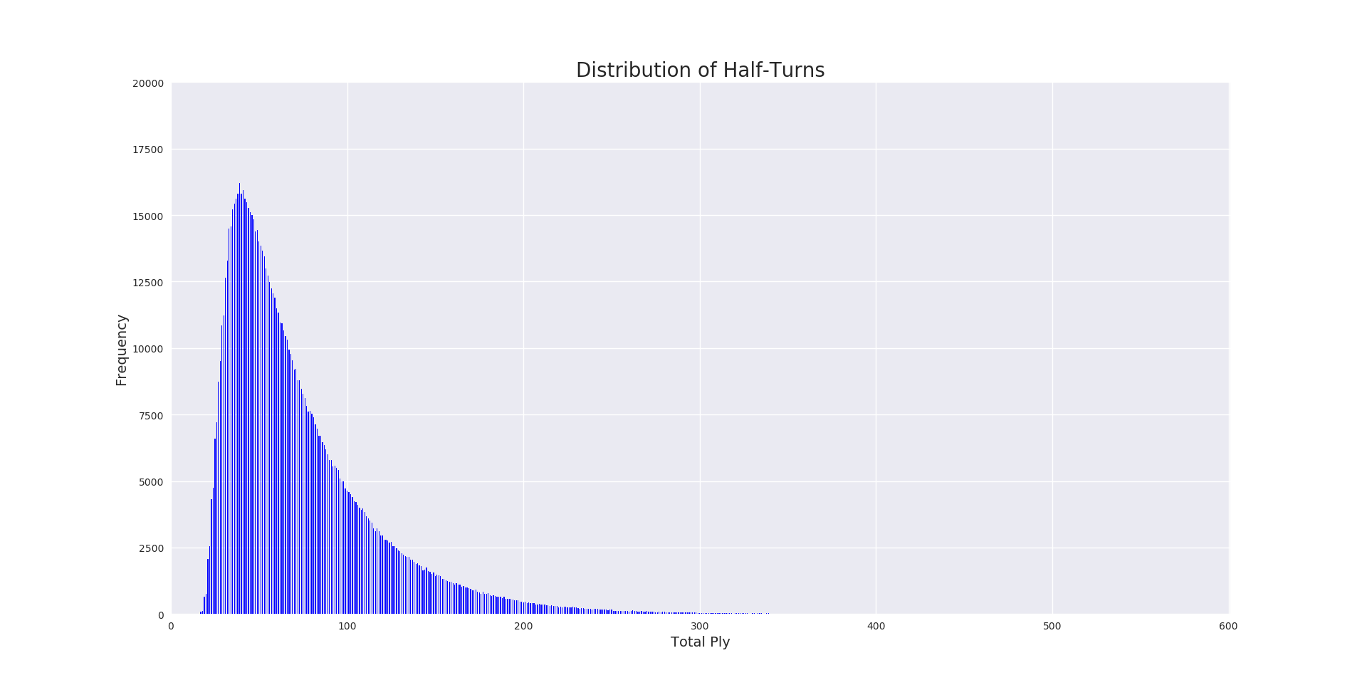
Looking next at the distribution of game lengths we see a neat pattern which peaks at 39 half-turns. The quickest game took only 17 ply, whilst the longest weighed in at 544! That’s 272 rolls of the die per player!

So this rounds up our brief look at Snakes and Ladders using Python. Just remember that not all research into games needs to be at the level of IBM’s Deep Blue in chess, or the recent successes of Demis Hassabis’s team on AlphaGo. For some games just a couple of dozen lines of code can yield insights and lead to discoveries that could help shape your strategy in future.

Speaking of which, next time Eva it’s my turn to go first!